
Mathematicians often isolate themselves within their specialties (the algebraic geometers vs the analysts vs the probabilists vs the theorists and so on). But some of the most brilliant results arise from applying tools from one field to problems in another.
One of the largest open problems in mathematics and computer science is the P vs NP problem. It asks whether a problem whose solution can be checked in polynomial time is actually solvable in polynomial time. You can learn the basics about P vs NP here. Since the problem was formalized by Stephen Cook in 1971, many people in complexity theory have spent their time trying to make progress on it. So why is P vs NP unsolved? Fundamentally, some people think that the problem cannot be proved or disproved from our standard set of mathematical assumptions (i.e P vs NP might be independent of ZFC and other axiomatic systems). Additionally, several proof techniques have been proven insufficient (specifically relativizing proofs and natural proofs).
(Debatably) The most viable track for progress on P vs NP that’s still on the table (for now, anyway) is actually rooted in algebra! The idea, introduced by Leslie Valiant in 1979, is to study two classes of polynomials, VP and VNP, and see whether they’re equal. (For those whose ears are ringing at that name, this is the same Valiant who would later come up with the “probably approximately correct” PAC learning model.) Many believe that a proof for whether or not VP equals VNP would be a huge step in solving P vs NP.
VP and VNP
To describe VP and VNP, we only need a few terms to classify some polynomials. Our multivariate polynomials will be over a field K, so just imagine the coefficients are real numbers, and in variables 


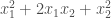
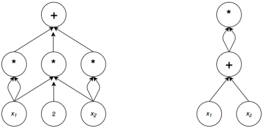
The size of an arithmetic circuit is the number of gates, the circles in the diagrams. The total complexity of a polynomial 


Now we’re ready to define the classes: VP is the class of families of polynomials for which
- the function mapping n to the degree of
- Most definitions also require that for
the minimum number of variables in the polynomial
is polynomially bounded. However this seems a consequence of
- Most definitions also require that for
Informally, VP is the class consisting of all families of polynomials which have polynomially bounded degree and complexity. So let’s see some examples and non examples:
- The family
is in VP.
- The family
is not in VP. While the polynomial can be computed in an arithmetic circuit of size
, the degree of
, which is not polynomially bounded.
- The determinant family,
, is the determinant of an
matrix with distinct indeterminate entries. The naïve arithmetic circuit has complexity
(see the definition for
below), but using Gaussian elimination on a matrix, the arithmetic circuit can be made to have size polynomial in
To refresh anyone’s memory on the determinant, for the 

More generally, for 


where 
VNP is the class of families of polynomials for which there exists a family ![g_n \in K[x_1,\cdots,x_{u(n)}]](https://s0.wp.com/latex.php?latex=g_n+%5Cin+K%5Bx_1%2C%5Ccdots%2Cx_%7Bu%28n%29%7D%5D&bg=ffffff&fg=404040&s=0&c=20201002)

In other words, given a monomial, so a term like 

- Any family in VP lies in VNP.
- The permanent family, denoted
, is the permanent of an
As a reminder, for the

and more generally for an

Looking at the sum definition for 
The permanent family is complete in VNP over all fields 


The big picture
The exact relation between P and VP or between NP and VNP should seem pretty hazy. After letting the definitions sink in, the analogs might “make sense” intuitively, but I’ve given no formal support as to why these are the “best” analogs. Or even why work on VP vs VNP gives insight to P vs NP. Some details for this are in section 9 of Valiant’s paper “Completeness Classes in Algebra“, but I’ll quote his first sentence from the section, and wave a hand at the technical details:
“… the formal Boolean analog of the previously defined algebraic notion of p-definability [functions in VNP] is closely related to the concept of nondeterminism as traditionally applied to discrete computations.”
So again, it’s not true that VP ≄VNP implies P ≄NP (although the converse is true), but the Boolean analogs of VP and VNP are closely related to P and NP, respectively.
P.S
After posting this a friend referred me to a survey by Scott Aaronson on the state of P vs NP. There’s a new (as of 2015) approach called Ironic Complexity Theory, which has been successful in proving circuit lower bounds. I plan on learning about this soon, but check out the survey for more information.

Nice intro!
> VPN is the class of families of polynomials for which there exists a family
I assume you mean VNP 😛
LikeLike
fixed! thanks!
LikeLike
The Algebraic Analog of P vs NP
I think the first determinant is wrong: x1*x7*x8, x7 and x1 are on the same column.
LikeLike
Ha, yep. Fixed it, thanks!
LikeLike